Data for aluminium from solid_data and thermooptic_data.
read`../therm_eq.m`:read`../therm_const.m`:read`../therm_proc.m`:with(therm_proc):with(plots):with(RealDomain):assume(t>0,tau>0):

>	su:="Aluminio_anodizado":dat:=[D=0.2*m_,delta=1e-3*m_,E=1360*W_/m_^2,R[GEO]=42100e3*m_,To=86164*s_,epsilon[p]=0.615,rho[p]=0.3,Tp=288.15*K_,Tinf=2.7*K_];dat:=op(dat),get_sol_data(su),Const,SI2,SI1:alpha=subs(dat,alpha);epsilon=subs(dat,epsilon);

The geostationary orbit (GEO) is so far (its radius is 6.6 times that of the Earth) that we can neglect thermal inputs from the planet. With data from planet_dat and VF-table ,the maximum values are:

>	eqF12:=Fsp=(1-sqrt(1-1/h^2))/2;eqh:=h=R[GEO]/R[T];eqh_:=evalf(subs(dat,%));eqF12_:=subs(eqh_,eqF12); Qp:=epsilon*A*Fsp*sigma*epsilon[p]*Tp^4;eqA:=A=Pi*D^2;eqA_:=evalf(subs(dat,%));Qp_:=subs(eqF12_,eqA_,dat,Qp);Qa_0:=alpha*A*Fsp*rho[p]*E;Qa_0_:=subs(eqF12_,eqA_,dat,%);

	(1)

i.e. the view factor from a small sphere at GEO to the Earth is Fsp=0.006 (i.e. only 0.6 % of the radiation outgoing from s impinges on p); the absorbed IR flux is Qp=0.14 W all around the orbit (Earth's emission is assumed uniform), and maximum albedo absorption is Qa_0=0.04 W, decreasing with orbit angle and being zero during eclipse.

The satellite geometry and GEO geometry at equinox make the thermal environment almost constant, except for the eclipse. The steady state temperature

>	eqEB:=m*c*dT/dt=Qs+'Qp'+Qa-Qinf;Qs:=alpha*Pi*D^2*E/4;Qs_:=subs(dat,Qs);Qinf:=epsilon*A*sigma*(T^4-Tinf^4);eqEB:=0=Qs-Qinf;Tst:=sqrt(sqrt(alpha*E/(4*epsilon*sigma)));Tst_:=evalf(subs(dat,SI0,Tst))*K_;'Tst_'=TKC(%);

	(2)

i.e. the sphere of anodized aluminium would attain 183 K (-90 ºC) when lit at steady state (a blackbody would reach 278 K; 5 ºC).

Taking orbit angle from the subsolar point, the eclipse period starts at (mind that our h is 1+h in that reference):

>	eq:=phi[es]=Pi-arccos(sqrt(h^2-1)/(h*cos(beta)));beta[equinox]=0;eq_:=evalf(subs(beta=0,eqh_,eq));phi[es]=evalf(rhs(%)*180*`º`/Pi)

	(3)

i.e. the eclipse starts at 2.99 rad and ends at 2*Pi-2.99=3.29 rad (i.e. it is in shadow from 171º until 189º). We need a multi-orbit variable to get a periodic evolution, but it may be good enough to solve the transient from the steady-state computed above, after entering the eclipse.

>

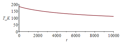
eqEBshadow:=m*c*dT/dt='Qp-Qinf';eqEBshadow:=A*delta*rho*c*diff(T(t),t)=-subs(T=T(t),Tinf=0,Qinf);sol:=dsolve(eqEBshadow,T(t))[1];C1:=solve(T0=subs(t=0,rhs(sol)),_C1);sol_:=subs(_C1=C1,sol);sol__:=subs(T0=Tst_,dat,SI0,%);plot(rhs(%),t=0..10000,T_K=0..200);Te:=To*(1-phi[es]/Pi);Te_:=subs(eq_,dat,%);Tee_:=subs(t=Te_,SI0,rhs(sol__))*K_;

	(4)

i.e. during the Te=4200 s that the eclipse lasts, the sphere temperature falls from Tst=183 K to Tee=136 K. From that on, solar radiation would heat up the sphere.

NOTE. This solution is more clear if in terms of the characteristic time, tau, such that:

>	sol:=T(t)=T0*(1/(1+t/tau)^(1/3));eqtau:=tau=delta*rho*c/(3*epsilon*sigma*''Tst''^3);eqtau_:=tau=evalf(subs(dat,SI0,rhs(eqtau)))*s_;Ttau:=subs(t=tau,T0='Tst',rhs(sol));Ttau_:=evalf(subs(t=tau,T0='Tst',rhs(sol)));Ttau__:=evalf(subs(t=tau,T0=Tst_,rhs(sol)));

	(5)

i.e. at the characteristic time, tau=2900 s, temperature has already fallen to 79 % (from 183 K to 145 K). As the eclipse lasts Te=4200 s, that means that the temperature of the sphere will fall appreciably, down to Tee=136 K, before the eclipse ends. Notice that, if the eclipse would last a very large time, the temperature would tend to Tinf=2.7 K (a bit more due to the heating from the planet, here neglected).

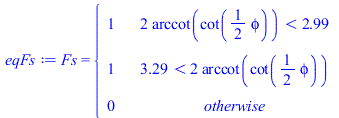
For the numerical simulation along the orbit (starting with the steady-state value Tst=183 K, although it does not matter, we start setting the time-Factor for solar irradiation:

>	eqEB:=m*c*diff(T(t),t)='Qs*Fs-Qinf';eqEB:=A*delta*rho*c*diff(T(t),t)=subs(T=T(t),Tinf=0,Qs*Fs-Qinf);phimod2pi:=proc(x,y) RETURN(arccot(cot(x*Pi/y))*y/Pi);end;eqFs:=Fs=piecewise(phimod2pi(phi,2*Pi)<rhs(eq_),1,phimod2pi(phi,2*Pi)>2*Pi-rhs(eq_),1,0);plot(rhs(%),phi=0..4*Pi,Fs=0..1);

and we change to angular variable (phi=2*Pi*t/To):

>

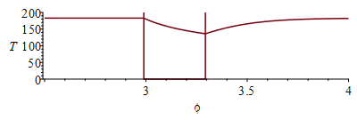
phi:='phi':eqEB:=A*delta*rho*c*Diff(T,phi)*2*Pi/To='Qs*Fs-Qinf';eqEB_:=subs(eqA_,T=T(phi),dat,SI0,%);sol_:=dsolve({subs(eqFs,eqEB_),T(0)=Tst_/K_},numeric,T(phi));odeplot(sol_,[phi,T(phi)],0..4*Pi); pl:=odeplot(sol_,[phi,T(phi)],2.5..4):pl0:=plot([[rhs(eq_),200],[rhs(eq_),0],[2*Pi-rhs(eq_),0],[2*Pi-rhs(eq_),200]]):display({pl,pl0});

i.e. we see that T(t) is constant from the subsolar point until entry into eclipse, then it falls from 183 K to 136 K, but as soon as it goes out it heats up towards the steady-state value.

>