>	restart:#"m13_p39"

Consider a circular-disc of radius R1=60 cm, thickness 1=5 mm, thermal capacity C1=500 J/K, painted white on the front and black on the rear. The disc acts as a sunshield to a coaxial spherical body of radius R2=0.5 m, black-painted, which is at a distance H=1 m between centres, and has a thermal capacity C2=15 kJ/K. Both objects are joined by a tubular pole made of aluminium with 1 cm external diameter and 0.3 mm wall thickness. The two objects are assumed to have high thermal conductivity and thus isothermal, constituting each one a node in the thermal problem. Find:

a) The global thermal capacity of the pole, to justify the simplification to two nodes (disc 1, and sphere 2).

b) All the view factors for the nodes.

c) The conductive and radiative couplings between nodes if all the surfaces are considered blackbodies.

d) The energy balance for the permanently aligned configuration Sun-disc-sphere in space (without nearby planets or moons), with the assumption of blackbodies.

e) The network equations in the real grey-body case.

Data:

>	read`../therm_eq.m`:read`../therm_const.m`:read`../therm_proc.m`:with(therm_proc):with(plots):

>	dat:=[R1=0.6*m_,C1=500*J_/K_,R2=0.5*m_,H=1*m_,C2=15e3*J_/K_,R3=0.005*m_,delta3=0.3e-3*m_,Es=1370*W_/m_^2,alpha[w]=0.20,epsilon[w]=0.85,epsilon[b]=0.90,rho3=2700*kg_/m_^3,c3=900*J_/(kg_*K_),k3=200*W_/(m_*K_)];dat:=op(dat),Const,SI2,SI1:

(1)

a) The global thermal capacity of the pole, to justify the simplification to two nodes (disc 1, and sphere 2).

>	C3:=m3*c3;C3:=rho3*2*Pi*R3*delta3*L*c3;L:=H-R2;C3_:=evalf(subs(dat,C3));

	(2)

This thermal capacity is much lower than the thermal capacities of the other two parts, so that, considering its small dimensions, it is not retained as a new node, and the sole influence in the thermal analysis is the conductive coupling between the two nodes considered.

b) All the view factors for the nodes.

>

eqF12:=F12=(4*r2^2)*(1-h/sqrt(1+h^2))/2;eqr2:=r2=R2/R1;eqr2_:=subs(dat,%);eqh:=h=H/R1;eqh_:=subs(dat,%);eqF12_:=subs(eqr2_,eqh_,eqF12);eqClosure:=F12+F10=1;eqRecipr:=A1*F12=A2*F21;eqF20:=F20=1-F21;eqF20:=F20=1-A1*F12/A2;eqA1:=A1=Pi*R1^2;eqA1_:=evalf(subs(dat,%));eqA2:=A2=4*Pi*R2^2;eqA2_:=evalf(subs(dat,%));eqF20_:=evalf(subs(eqA1_,eqA2_,eqF12_,eqF20));

	(3)

i.e. the external face of the disc only sees the background (F1e,0=1; the Sun is just a point), the internal face of the disc sees the sphere with F1i,2=0.20 and the background with F1i,0=1-F1i,2=1-0.20=0.80. Finally, the sphere sees the disc with F2,1=A1F1i,2/A2=0.072 and the background with F2,0=1-F2,1=1-0.07=0.93.

Notice that A1 only refers to one side of the disc.

c) The conductive and radiative couplings between nodes if all the surfaces are considered blackbodies.

For blackbody surfaces the radiative coupling, excluding sigma, is R21=A2·F21 (other times it is defined to include the constant sigma).

>	Qcod21:=K21*(T2-T1);K21:='k3*2*Pi*R3*delta3/L';K21_:=subs(dat,evalf(subs(dat,%)));Qrad21:=sigma*R21*(T2^4-T1^4);Qrad21:=sigma*A2*F21*(T2^4-T1^4);

	(4)

d) The energy balance for the permanently aligned configuration Sun-disc-sphere in space (without nearby planets or moons), with the assumption of blackbodies.

>

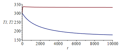
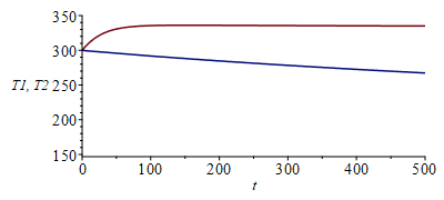
eqEB1:=C1*diff(T1(t),t)=A1*Es+'k3*2*Pi*R3*delta3*(T2(t)-T1(t))/L'+sigma*A1*F12*(T2(t)^4-T1(t)^4)+sigma*A1*F1i0*(Tinf^4-T1(t)^4)+sigma*A1*F1e0*(Tinf^4-T1(t)^4);eqEB1_:=evalf(subs(eqA1_,eqA2_,F1i0=1-F12,F1e0=1,eqF12_,Tinf=0,dat,SI0,%));eqEB2:=C2*diff(T2(t),t)=-'k3*2*Pi*R3*delta3*(T2(t)-T1(t))/L'-sigma*A1*F12*(T2(t)^4-T1(t)^4)+sigma*A2*F20*(Tinf^4-T2(t)^4);eqEB2_:=evalf(subs(eqA1_,eqA2_,eqF20_,eqF12_,Tinf=0,dat,SI0,%));sol_:=dsolve([eqEB1_,eqEB2_,T1(0)=300,T2(0)=300],numeric);odeplot(sol_,[[t,T1(t)],[t,T2(t)]],0..1e4,view=[0..1e4,150..350]);odeplot(sol_,[[t,T1(t)],[t,T2(t)]],0..500,view=[0..500,150..350]);st_:=sol_(1e5):T1st_:=op(2,(op(2,st_)))*K_;T2st_:=op(2,(op(3,st_)))*K_;

	(5)

The final steady state can be found by solving the above equations with dT/dt=0, with the result T1()=332 K, T2()=172 K. Notice the different transient times of the nodes, due to different thermal capacities; node 1 has very low thermal inertia and equilibrates in a hundred of seconds, while node 2 takes several hours to equilibrate. In fact, node 2 is initially so hot that node 1 first stabilises to 336 K before finally reaching the 332 K in the long run.

It is instructive to compute the heat rates exchanged in the steady state.

>	Qs:=A1*Es;Qs_:=subs(eqA1_,dat,%);Qcod12:='k3*2*Pi*R3*delta3*(T1st_-T2st_)/L';Qcod12_:=subs(dat,evalf(subs(dat,%)));Qrad12:=sigma*A1*F12*'(T1st_^4-T2st_^4)';Qrad12_:=subs(eqF12_,eqA1_,dat,%);

	(6)

i.e., the disc gets 1550 W from the Sun, and transmits 143 W by radiation to the sphere (plus 0.6 W by conduction through the pole).

e) The network equations in the real grey-body case.

Instead of writing the energy balance equation as dE/dt=W+Qcond+Qrad, it is better to set it as Qrad=dE/dt-W-Qcond. Besides, one must choose one node at each ‘uniform’ surface in the radiative enclosure, so that we are forced to separate node 1 in node 1e and node 1i, each with half the total thermal capacity and conductively connected through a high enough conductance to make the difference in temperature negligible.

The simplification of this initial electrical-analogy circuit shown in Fig. 2 reduces to system to 4 equation with 4 unknowns (M1,bb,M1i,M2,M2,bb):

>

eqNet1b:=(0-sigma*T1^4)/(1/(A1*1)+(1-epsilon[w])/(A1*epsilon[w]))+(M1i-sigma*T1^4)/((1-epsilon[b])/(A1*epsilon[b]))=C1dT1_dt-alpha[w]*A1*Es-K12*(T2-T1);eqNet1i:=(sigma*T1^4-M1i)/((1-epsilon[b])/(A1*epsilon[b]))+(M2-M1i)/(1/(A1*F12))+(0-M1i)/(1/(A1*F10))=0;eqNet2:=(M1i-M2)/(1/(A1*F12))+(sigma*T2^4-M2)/((1-epsilon[b])/(A2*epsilon[b]))+(0-M2)/(1/(A2*F20))=0;eqNet2b:=(M2-sigma*T2^4)/((1-epsilon[b])/(A2*epsilon[b]))=C2dT2_dt-K12*(T1-T2);

	(7)

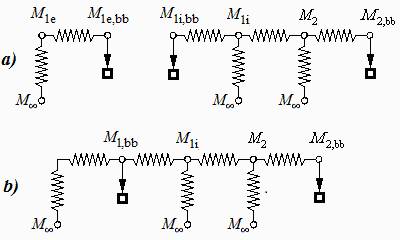
Fig. 2. a) Initial electrical-analogy circuit, and a network simplification.

And we can extract the intermediate variables M2 and M1i from the last two equations and substitute in the other two, to leave a system of 2 equations with 2 unknowns (T1 and T2), which have to be solved numerically because of the non-linearity.

>	M2_:=solve(eqNet2b,M2);M1i_:=solve(subs(M2=M2_,eqNet2),M1i):eqNet1b_:=subs(M2=M2_,M1i=M1i_,eqNet1b):eqNet1i_:=subs(M2=M2_,M1i=M1i_,eqNet1i): #LONG equations

(8)

The numerical expressions are:

>	eqs:=subs(eqA1_,eqA2_,F10=1-F12,eqF12_,eqF20_,K12=K21_,dat,SI0,[eqNet1b_,eqNet1i_]);

(9)

Steady solution (you may check with alpha=epsilon=1 that we recover T1=332 K and T2=172 K.

>	fsolve(subs(C1dT1_dt=0,C2dT2_dt=0,eqs),{T1,T2},{T1=100..400,T2=100..400});

(10)

Transients:

>

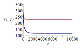
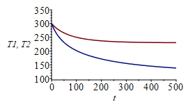
eqs_:=[op(subs(T1=T1(t),T2=T2(t),C1dT1_dt=C1*diff(T1(t),t),C2dT2_dt=C1*diff(T2(t),t),dat,SI0,eqs)),T1(0)=300,T2(0)=300];sol_:=dsolve(eqs_,numeric);odeplot(sol_,[[t,T1(t)],[t,T2(t)]],0..1e4,view=[0..1e4,100..350]);odeplot(sol_,[[t,T1(t)],[t,T2(t)]],0..500,view=[0..500,100..350]);st_:=sol_(1e5):T1st_:=op(2,(op(2,st_)))*K_;T2st_:=op(2,(op(3,st_)))*K_;

	(11)

where we see the tendency towards the steady state with 230 K at the disc and 116 K at the sphere.

The lesson to learn is that the network formulation of radiative problems with partially-reflecting surfaces is cumbersome (and this is not valid for partial specular reflection or partially-transparent media).

>