>	restart:#"m16_p31"

>	read`../therm_chem.m`:with(therm_chem);with(therm_proc):

A thermodynamic simulation of a reciprocating engine cycle is to be performed using a Weibe-function to model the combustion process, with typical parameters for a SI-ICE: a=5, m=3,  bs=-10º,  bs=-70º. The model is to be applied to a Yamaha YZ250FN four-stroke 250 cc motorcycle, single cylinder, spark-ignition engine, with the following dimensions: bore D=0.0770 m, stroke L=0.0526 m, with a compression ratio r=12.5. Only the compression and expansion strokes are to be considered, with the crank angle,  , as the independent variable, and only at the steady-state corresponding to full load at 8500 rpm, i.e., assume the cylinder initially filled with an stoichiometric octane/air mixture at ambient conditions (unit volumetric efficiency). Perform:

a) Compute the displacement volume, clearance volume, trapped mass of air and fuel, and chemical energy released per cycle.

b) Compute gas volume and energy release as a function of   and make a plot.
c) Establish the energy balance for the gas, and get a single differential equation to compute the pressure profile p( ).
d) Solve numerically for p( ), T( ) and dWsh/d  (the contribution to the shaft work at each step). Plot them.
e)      Compute the shaft power and the energy efficiency of the engine.

Data:

>	su1:="Aire":fuel:=C8H18;dat:=[D=0.0770*m_,L=0.0526*m_,Vd=249e-6*m_^3,r=12.5,N=(8500/60)/s_,a=5,m=3,theta_bs=-10*Pi/180,theta_bd=60*Pi/180,b=3]:evalf(%,3);

Sketch and nomenclature:

Fig. 1. Crank angle diagram showing enclosed volume in m³ (red line), its angle derivative (gree line), and valve controls and burning timing (in black).

D=bore

L=stroke

Vcl=clearance volume

Vd=displacement volume

b=Lrod/(L/2) (of order 2)

ivc=intake valve closes

evo=exhaust valve opens

bs=burning startup

bd=burning duration

Eqs. const.:

>	Adat:=get_gas_data(su1):dat:=op(dat),op(subs(g=g0,[Const])),SI2,SI1:

Slider and Crank-Shaft mechanism (a typical connecting rod / crank shaft length ratio =3 has been used):

>

eqCS:=V=Vcl+Vd*(sqrt(b^2-sin(theta)^2)+1-cos(theta)-b)/2;eqCS_diff:='V_theta=diff(rhs(eqCS),theta)';eqWeibe:=Qacc=Qcycle*(1-exp(-a*((theta-theta[bs])/theta[bd])^m));eqWeibe_diff:=Qacc_theta='diff(rhs(eqWeibe),theta)';eqWeibe_diff:=Qacc_theta=diff(subs(theta[bs]=theta_bs,theta[bd]=theta_bd,rhs(eqWeibe)),theta):

a)Compute the displacement volume, clearance volume, trapped mass of air and fuel, and chemical energy released per cycle.

>

eqDAT_check_Vd:=Vd=L*Pi*D^2/4;eqDAT_check_Vd_:=(Vd-L*Pi*D^2/4)/Vd=evalf(subs(dat,(Vd-L*Pi*D^2/4)/Vd),4);eqr:=r=(Vcl+Vd)/Vcl;'Vcl'=solve(%,Vcl);Vcl_:=subs(dat,solve(eqr,Vcl)):'Vcl'=evalf(%,2);ma:=rho*(Vcl+Vd);ma:=p0*(Vcl+Vd)/(R*T0);ma_:=subs(Vcl=Vcl_,Adat,dat,ma):'ma'=evalf(%,2);Ateo(fuel):A0_:=rhs(%):A[0]=evalf(%,2)*mol_A/mol_F;A0m_:=subs(Adat,A0_*M/rhs(Mf(fuel))):A[0]=evalf(%,3)*kg_A/kg_F;mF:='ma/A[0]';mF_:=ma_/A0m_:'mF'=evalf(%,2);Qcycle_:='mF*PCI';eqST:=eq_fit(fuel+a*O2=b*CO2+c*H2O);PCI_:=PCI(eqST);PCIm_:=subs(PCI_/rhs(Mf(fuel))):'PCI'=evalf(%,2);PCIm_:=46e6*J_/kg_:Qcycle_:=mF_*PCIm_;plot(subs(eqCS,eqCS_diff,Vcl=Vcl_,dat,SI0,[V,V_theta]),theta=-Pi..Pi);

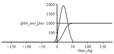
b) Compute gas volume and energy release as a function of   and make a plot

>

Qacc_otto:=piecewise(theta<0,0,Qcycle);Qacc_:=piecewise(theta<theta_bs,0,theta>theta_bs+theta_bd,Qcycle,rhs(eqWeibe));Qacc_theta_:=diff(Qacc_,theta):Qacc_theta_:=piecewise(theta<theta_bs,0,theta>theta_bs+theta_bd,0,rhs(eqWeibe_diff)):uc:=180/Pi;plot(subs(Qcycle=Qcycle_,theta[bs]=theta_bs,theta[bd]=theta_bd,Vcl=Vcl_,dat,SI0,theta=theta_deg/uc,{Qacc_otto,Qacc_,Qacc_theta_}),theta_deg=-Pi*uc..Pi*uc,Qdot_and_Qacc=0..2000,color=black);

c) Establish the energy balance for the gas, and get a single differential equation to compute the pressure profile p( ).

The real combustion process is assimilated to a heat transfer process (i.e. DUtherm+DUchem=W+0 to DUtherm=W+Q).

>

eqEB:='ma'*c[va]*Diff(T,theta)=Diff(Q,theta)-p(theta)*Diff(V,theta);eqIGM:=p*V=m*R*T;eqIGM:=diff(p(theta),theta)/p(theta)+diff(V(theta),theta)/V(theta)=diff(T(theta),theta)/T(theta);eqIGM:=dp_dt_p+dV_dt_V=dT_dt_T;dV_dt_V:=V_theta/V;dV_dt_V:=subs(Vcl=Vcl_,dat,eqCS,eqCS_diff,V_theta/V);dT_dt:='(Qacc_theta-p*V_theta)/(ma*c[va])';dT_dt_T:=dT_dt*ma*R/(p*V);eqIGM:=dp_dt_p='dT_dt_T-dV_dt_V';eqDp:=diff(p(theta),theta)=p(theta)*subs(p=p(theta),dT_dt_T-dV_dt_V);eqDp_:=evalf(subs(Qacc_theta=Qacc_theta_,eqCS,eqCS_diff,Vcl=Vcl_,Qcycle=Qcycle_,theta[bs]=theta_bs,theta[bd]=theta_bd,c[va]=c[v],Adat,dat,SI0,eqDp)):

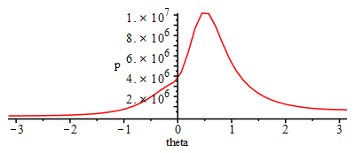
d) Solve numerically for p( ), T( ) and dWsh/d  (the contribution to the shaft work at each step). Plot them.

Direct plot

>	dsol1 := dsolve({eqDp_,p(-Pi)=1e5}, numeric, p(theta),range=-Pi..Pi);with(plots):odeplot(dsol1,theta=-Pi..Pi);dsol1(0),p(0)=op(2,op(2,dsol1(0))):evalf(%);

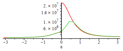
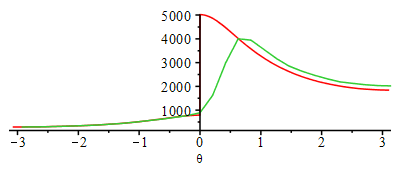
But, before detailed plots are presented, the ideal Otto cycle is worked out for comparison with Weibe model.

>

p12:=p0*((Vcl+Vd)/V)^gamma;T12:=T0*((Vcl+Vd)/V)^(gamma-1);p2_:=subs(V=Vcl,Vcl=Vcl_,Adat,dat,p12):'p2'=evalf(%,2);T2_:=subs(V=Vcl,Vcl=Vcl_,Adat,dat,T12):'T2'=evalf(%,2);DT23:='mF*PCI/(ma*c[va])';T3_:=subs(Adat,dat,T2_+mF_*PCIm_/(ma_*c[v])):'T3'=evalf(%,3);p3:='ma*R*T3/Vcl';p3_:=subs(Adat,dat,ma_*R*T3_/Vcl_):'p3'=evalf(%,2);p34:='p3*(Vcl/V)^gamma';T34:='T3*(Vcl/V)^(gamma-1)';p4_:=subs(T3=T3_,V=Vcl+Vd,Vcl=Vcl_,Adat,dat,p34):'p4'=evalf(%,2);T4_:=subs(T3=T3_,V=Vcl+Vd,Vcl=Vcl_,Adat,dat,T34):'T4'=evalf(%,3);potto:=subs(T3=T3_,p3=p3_,eqCS,Vcl=Vcl_,Adat,dat,piecewise(theta>0,p34,p12)):Totto:=subs(T3=T3_,p3=p3_,eqCS,Vcl=Vcl_,Adat,dat,piecewise(theta>0,T34,T12)):Wu_otto:='(potto-p0)*Diff(V,theta)';Wu_otto:=subs(eqCS_diff,dat,(potto-p0)*V_theta):plot(subs(SI0,Wu_otto),theta=-Pi..Pi):

Ni=Number of intervals for discretization of crank-angle. For debugging: #print(evalf([theta_(i),p_(i),V_(i),T_(i),Wu_(i)]))

>

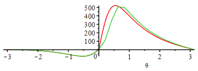
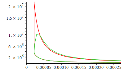
Ni:=30:Dtheta:='2*Pi/Ni';for i from 1 to Ni do theta_(i):=-Pi+2*Pi*i/Ni;p_(i):=op(2,op(2,eval(subs(theta=theta_(i),dsol1(theta)))))*Pa_; V_(i):=subs(Vcl=Vcl_,dat,theta=theta_(i),rhs(eqCS)); T_(i):=subs(Adat,dat,p_(i)*V_(i)/(ma_*R));Wu_(i):=subs(dat,(p_(i)-p0)*subs(eqCS_diff,theta=theta_(i),V_theta));od: plot(subs(SI0,{potto,[seq([theta_(i),p_(i)],i=1..Ni)]}),theta=-Pi..Pi);plot(subs(SI0,{Totto,[seq([theta_(i),T_(i)],i=1..Ni)]}),theta=-Pi..Pi);plot(subs(SI0,{Wu_otto,[seq([theta_(i),Wu_(i)],i=1..Ni)]}),theta=-Pi..Pi);plot(subs(eqCS,Vcl=Vcl_,dat,SI0,{[V,potto,theta=-Pi..Pi],[seq([V_(i),p_(i)],i=1..Ni)]}),0..subs(dat,SI0,Vcl_+Vd));loglogplot(subs(eqCS,Vcl=Vcl_,dat,SI0,{[Totto,potto,theta=-Pi..Pi],[seq([T_(i),p_(i)],i=1..Ni)]}),'T_K'=300..5000,'p_Pa'=1e5..2.5e7);

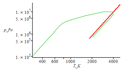HINT: if no fuel is added (put 0*mF), the plots would correspond to isentropic compression and expansion, with maximum values of p(0)=p0*r^gamma and T(0)=T0*r^(gamma-1).

e) Compute the shaft power and the energy efficiency of the engine.

>

Wu:=Int(p-p0,V);Wu:=Int((p-p0)*V_theta,theta);i:='i':Wu_cycle_:=subs(dat,evalf(sum(Wu_(i)*eval(Dtheta),i=1..Ni))):'Wu_cycle'=evalf(%,2);pMEP:='Wu_cycle/Vd';pMEP_:=subs(dat,Wu_cycle_/Vd):'pMEP'=evalf(%,3);Wu_dot:='Wu_cycle*N/(Nstrokes/2)';Wu_dot_:=subs(dat,Wu_cycle_*N/2):'Wu_dot'=evalf(%,2);eta[e]:='Wu_cycle/Qcycle';eta[e]:=Wu_cycle_/Qcycle_:'eta[e]'=evalf(%,2);SFC:=mF_/Wu_cycle_:%*(1000*g_/kg_)*(3.6e6*J_/kWh_):'SFC'=evalf(%,2);eta[Otto]:=1-1/r^(gamma-1);etaO_:=evalf(subs(Adat,dat,%)):'eta[Otto]'=evalf(%,2);Wu_cycle_Otto:='eta[Otto]*Qcycle';etaO_*Qcycle_:Wu_cycle_Otto:=evalf(%,2);

Too high efficiency (too low specific fuel consumption). The reasons why this engine model predicts such a high efficiency is because we did not consider unburnt fuel (some 5%), engine friction (some 5% at full load), fluid pumping work to renovate gases (some 2%), fluid loses around piston rings (some 1%), and heat transfer through the cylinder walls (<1%), have not been taken into account.

ADDITIONAL DATA. The 250cc Yamaha engine has a rough external measurement of .35 x .41 x .51 meters, not including the exhaust system, i.e. some 73 litres in volume, with an approximate dry weigh of 27 kg including a 5-speed transmission and cooling pump. Its specific fuel consumption is SFC=330 g/kWh, and maximum power is 30.5 kW.