| > | restart:#"m13_p34" |
Consider a spherical black-body of 1 m in diameter, in an equatorial orbit at 300 km (LEO), and at GEO. Find:
a) Orbital period.
b) Eclipse duration.
c) Solar input along the orbit.
d) Infrared input from the planet, assumed at a temperature of 288 K and with =0.6.
e) Albedo input along the orbit, assuming an albedo of 0.3 and a simple albedo model.
f) Periodic temperature evolution, assuming the body is isothermal and has a mass of 100 kg with an average thermal capacity of 1000 J/(kg·K)..
Data:
| > | read`../therm_eq.m`:read`../therm_const.m`:read`../therm_proc.m`:with(therm_proc):with(plots): |
| > | dat:=[D=1*m_,R=6370e3*m_,E=1370*W_/m_^2,H_LEO=300e3*m_,H_GEO=35.8e6*m_,G=6.67e-11*N_*m_^2/kg_^2,M=5.97e24*kg_,Tp=288*K_,epsilon=0.6,rho=0.3,m=100*kg_,c=1000*J_/(kg_*K_)]; |

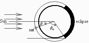
Fig. 1. a) Lateral view of equatorial orbits. b) Orbit view from the North Pole, to show the angular potion origin along the orbit, and the eclipse period (in black).
| > | dat:=op(dat),Const,SI2,SI1: |
a) Orbital period.
From orbital mechannics:
| > | Orbit_period:=T=2*Pi*sqrt(a^3/(G*M));a=R+H;T_LEO:=subs(SI2,evalf(subs(a=R+H_LEO,dat,Orbit_period)));T_GEO:=subs(SI2,evalf(subs(a=R+H_GEO,dat,Orbit_period))); |
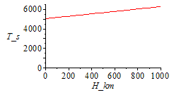
i.e. the LEO period is 5400 s (90 min), and GEO period 86200 s (23 h 58 min). Notice that the influence of H in LEO is not great, and that the GEO altitude can be computed from orbital mechanics knowing that its period is a sideral day (roughly 24 h).
| > | plot(subs(a=R+1000*H_km,dat,SI0,rhs(Orbit_period)),H_km=0..1000,T_s=0..6500); |
 |
Notice that we do not need to find G and M, since the GM-product can be found from g and R by the relations:
| > | eqG:=F=G*M*m/R^2;eqg:=F=m*g;eqGg:=g=G*M/R^2;eqGg_:=subs(dat,%); |
b) Eclipse duration.
The eclipse duration depends on the inclination of the equatorial plane to the ecliptic. Maximum duration occurs when the Sun is in the equatorial plane, i.e. at the equinocces.
We only consider one orbit (phi=0..360º from subsolar point), and only this maximum eclipse duration (with Fig. 1).
| > | Eclipse_start:=phi[es]=Pi/2+arccos(R/(R+H));Eclipse_start:=phi[es]=Pi-arcsin(R/(R+H));Eclipse_fraction:=T[e]/T[o]=expand(1-rhs(Eclipse_start)/Pi);LEO_es:=phi_es=evalf(subs(H=H_LEO,dat,rhs(Eclipse_start)));LEO_es_deg:=phi_es=evalf(rhs(%)*180/Pi)*'º';LEO_ee:=phi_ee=evalf(2*Pi-rhs(LEO_es));LEO_ee_deg:=phi_ee=evalf(360*º-rhs(LEO_es_deg));LEO_ef:=evalf(subs(H=H_LEO,dat,Eclipse_fraction));LEO_ed:=rhs(%)*rhs(T_LEO);GEO_es:=phi_es=evalf(subs(H=H_GEO,dat,rhs(Eclipse_start)));GEO_es_deg:=phi_es=evalf(rhs(%)*180/Pi)*'º';GEO_ee:=phi_ee=evalf(2*Pi-rhs(GEO_es));GEO_ee_deg:=phi_ee=evalf(360*º-rhs(GEO_es_deg));GEO_ef:=evalf(subs(H=H_GEO,dat,Eclipse_fraction));GEO_ed:=rhs(%)*rhs(T_GEO); |
i.e. the LEO eclipse, which starts 107º after the subsolar point, lasts 40% of the orbit (2200 s, 37 min), whereas the GEO eclipse, which starts 171º after the subsolar point, only lasts 5% of the orbit, but this amounts to 4160 s (69 min, 72 minutes including the penumbra, nearly double than in LEO).
Notice that the above computations refer only to maximum values, which occur at 20 March and 22 September. LEO eclipse duration varies little with the season (i.e. with solar declination), but in GEO the influence is great: there are only GEO eclipses near the equinocces (when solar declination <8.7º, Fig. 1, which occurs from 27-Feb to 11-Apr and from 28-Aug to 11-Oct).
c) Solar input along the orbit.
The energy absorbed (or 'heat input') is constant when sunlit, and zero in eclipse.
We must set up a step function to signal eclipses. In order for it to be valid for angles beyond 2*Pi, it is worth setting a function to wrap up any angle to the 0..2*Pi interval.
| > | Qs:=alpha*Afrontal*E*Fs;p:=proc(phi) evalf(2*Pi*frac(phi/(2*Pi)));end;Fs:=piecewise(p(phi)<phi_es,1,p(phi)>(2*Pi-phi_es),1,0);plot(subs(phi_es=rhs(LEO_es),phi_ee=rhs(LEO_ee),Fs),phi=0..2*Pi,Fs_LEO=0..1);plot(subs(phi_es=rhs(GEO_es),phi_ee=rhs(GEO_ee),Fs),phi=0..2*Pi,Fs_GEO=0..1);Qs_max:=Afrontal*E;Afrontal:=(Pi*D^2/4);Qs_max_:=subs(dat,evalf(subs(dat,Qs_max))); |
 |
 |
 |
i.e. the 1 m in diameter spherical blackbody gets 1076 W directly from the Sun, when lit, zero otherwise.
d) Infrared input from the planet, assumed at a temperature of 288 K and with =0.6.
If the planet is assumed isothermal, the infrared input is constant along the orbit. The view factor from a small sphere to a much larger sphere is found in View factor tabulations.
| > | Qp:=alpha*A*Fbp*epsilon*sigma*Tp^4;A:=Pi*D^2;Fbp:=(1-sqrt(1-1/h^2))/2;eqh:=h=(H+R)/R;LEOh:=subs(H=H_LEO,dat,eqh);GEOh:=subs(H=H_GEO,dat,eqh);Fbp_LEO:=subs(LEOh,Fbp);Fbp_GEO:=subs(GEOh,Fbp);Qp_LEO:=subs(dat,evalf(subs(alpha=1,LEOh,dat,Qp)));Qp_GEO:=subs(dat,evalf(subs(alpha=1,GEOh,dat,Qp))); |
i.e. IR inputs are 259 W at LEO and 4 W at GEO.
e) Albedo input along the orbit, assuming an albedo of 0.3 and a simple albedo model.
Maximum albedo input occurs at subsolar position and is Qa_max:=alpha*A*Fbp*rho*E.
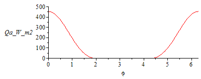
For the variation of albedo input with orbit angle, a simple model may be that it is proportional to the lit area seen (i.e. the crescent) squared (to account for the fact that the smaller the crescent, the smaller the irradiance got per normal surface). However, as the fraction of lit area seen depends on orbit altitude, a simpler model may be to compute the crescent area from afar (i.e. its orthogonal proyection) and multiply it (its square) by a parabolic function that ends at the eclipse; namely:
| > | Qa_max:=alpha*A*Fbp*rho*E;Qa_max_LEO:=subs(dat,evalf(subs(alpha=1,LEOh,dat,Qa_max)));Qa_max_GEO:=subs(dat,evalf(subs(alpha=1,GEOh,dat,Qa_max)));Fcrescent:=(1+cos(phi))/2;Fa:=Fcrescent^2*piecewise(p(phi)<phi_es,(1-(p(phi)/phi_es)^2),p(phi)>(2*Pi-phi_es),(1-((2*Pi-p(phi))/phi_es)^2),0);Qa:='Qa_max*Fa';plot(subs(alpha=1,LEOh,LEO_es,dat,SI0,Qa),phi=0..2*Pi,Qa_W_m2=0..500);plot(subs(alpha=1,GEOh,GEO_es,dat,SI0,Qa),phi=0..2*Pi,Qa_W_m2=0..10); |
 |
 |
 |
Notice that planet effects (IR and albedo) can be neglected at very high orbits like GEO.
f) Periodic temperature evolution, assuming the body is isothermal and has a mass of 100 kg with an average thermal capacity of 1000 J/(kg·K)..
The energy balance is dE/dt=W+Q=0+Qs+Qa+Qp-Qout, since there is no mechanical or electrical work. For instance, in the LEO case:
| > | eqEB:=dE/dt=Q[net,inp]-Q[net,out];eqEB:=m*c*diff(T(t),t)=Qs+Qa+Qp-A*sigma*T(t)^4:eqEB_:=subs(alpha=1,LEOh,LEO_es,Afrontal=A/4,dat,SI0,eqEB); |
  |
a first-order ordinary differential equation which must be solved with some initial conditions (e.g. T(0)=300 K) until transients decay and a periodic solution remains.
This can be done by Euler's method or better by some Runge-Kutta method.
Let us run the numerical simulation for N=5 orbits, with Dt=100 s, starting with T0=300 K. The number of discrete t-points are N*Tperiod/Dt.
| > | To:=subs(SI0,rhs(T_LEO));N:=5;Dt:=100;TE[1]:=300;Np:=round(N*To/Dt);for i from 1 to Np-1 do TE[i+1]:=TE[i]+evalf(subs(phi=2*Pi*Dt*i/To,alpha=1,LEOh,LEO_es,Afrontal=A/4,dat,SI0,Dt*(Qs+Qa+Qp-A*sigma*TE[i]^4)/(m*c)));od:plEuler:=plot([seq([Dt*i,TE[i]],i=1..Np)]):sol_:=dsolve([evalf(subs(phi=2*Pi*t/To,SI0,eqEB_)),T(0)=300],type=numeric,range=0..N*To);plRunge:=odeplot(sol_,color=black):display([plEuler,plRunge]); |
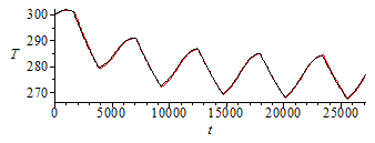 |
We see the 5th orbit is already periodic and plot it aside (notice that the initial and final T-values must coincide to be periodic, but this is not the mean temperature, Tmean.
| > | i:='i':Tmean:=sum(TE[i],i=round(Np*(N-1)/N)..Np)/(Np+1-round(Np*(N-1)/N));Tnax:=max(seq(TE[i],i=round(Np*(N-1)/N)..Np));Tnin:=min(seq(TE[i],i=round(Np*(N-1)/N)..Np));plmean:=plot([[0,Tmean],[N*To,Tmean]]):display([plEuler,plRunge,plmean],view=[(N-1)*To..N*To,250..300]); |
 |
i.e, once in periodic state, the body temperature oscillates between 268 K and 284 K with a period average of 276 K (i.e. between -5 ºC and 11 ºC, with a mean of 3 ºC).
In the case of GEO
| > | To_:=subs(SI0,rhs(T_GEO));N_:=3;Dt_:=1000;TE_[1]:=300;Np_:=round(N_*To_/Dt_);for i from 1 to Np_-1 do TE_[i+1]:=TE_[i]+evalf(subs(phi=2*Pi*Dt_*i/To_,alpha=1,GEOh,GEO_es,Afrontal=A/4,dat,SI0,Dt_*(Qs+Qa+Qp-A*sigma*TE_[i]^4)/(m*c)));od:plEuler_:=plot([seq([Dt_*i,TE_[i]],i=1..Np_)]):sol_:=dsolve([evalf(subs(phi=2*Pi*t/To_,alpha=1,GEOh,GEO_es,Afrontal=A/4,dat,SI0,eqEB)),T(0)=300],type=numeric,range=0..N_*To_);plRunge:=odeplot(sol_,color=black):display([plEuler_,plRunge]);i:='i':Ni_:=round(Np_*(N_-1)/N_);Tmean:=sum(TE_[i],i=Ni_..Np_)/(Np_+1-Ni_);Tnax:=max(seq(TE_[i],i=Ni_..Np_));Tnin:=min(seq(TE_[i],i=Ni_..Np_));plmean:=plot([[0,Tmean],[N_*To_,Tmean]]):display([plEuler_,plRunge,plmean],view=[(N_-1)*To_..N_*To_,240..300]); |
 |
 |
Notice how pronunced the effect of eclipse may be (and how much Euler's solution departs from the more accurate R-K) on geostationary orbits (fortunately, there are only GEO eclipses near the equinocces, as wxplained above, contrary to LEO, where eclipse duration varies little with season).
| > |
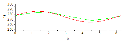
Comparison with the linear sinusoidal approximation for LEO: Tlin=275+10.8*cos(phi-1.32) in [K], corresponding to a sinusoidal input (Qs_max_+Qa_max_LEO)*(1+cos(phi))/2+Qp.
| > | TlinLEO:=275+10.8*cos(phi-1.32);plEuler_:=plot([seq([2*Pi*(Dt*i-(Np-54)*Dt)/5429,TE[i]],i=Np-54..Np)],color=green):plin:=plot(TlinLEO,phi=0..2*Pi,'T'=250..300):display([plEuler_,plin],view=[0..2*Pi,250..300]);plot(subs(alpha=1,LEOh,LEO_es,dat,SI0,[(Qs_max_+Qa_max_LEO)*(1+cos(phi))/2+Qp,(Qs+Qa+Qp)]),phi=0..2*Pi,Q=0..2000); |
 |
 |
The great advantage of this approximation is that it can be analytically solved.
| > |