| > | restart:#"m13_p24" |
| > | read`../therm_const.m`:read`../therm_proc.m`:read`../therm_eq.m`:with(therm_proc):with(RealDomain):with(plots):assume(t>0,tau>0): |
Consider a panel of 1·0.5·0.01 m¬3 deployed from a spacecraft orbiting Mars (at 1.5 AU from the Sun) at the subsolar position and 300 km altitude, with its face-normal tilted 30º to sun rays. Neglect the effects of other parts of the spacecraft, and assume the panel is painted black on the face looking down the planet and white on the other face; take for the bulk properties of the panel =50 kg/m3, c=1000 J/(kg·K), and k=0.01 W/(m·K). Find:
a) The solar irradiance and the power absorbed from the Sun.
b) The heat loads from the planet.
c) The power emitted by the plate, assuming the whole plate is at temperature T0, and in the case of different temperatures at each face, T1 and T2.
d) The steady value of T0, T1 and T2 under the above conditions.
e) The temperature evolution after entering into eclipse (assuming the above T0 as initial state).
Data:
| > | dat:=[A=1*0.5*m_^2,delta=0.01*m_,r=1.5,H=300e3*m_,beta=evalf(30*Pi/180),alpha1=0.2,alpha2=0.95,epsilon1=0.85,epsilon2=0.9,R=3.4e6*m_,Tp=217*K_,rhop=0.15,epsilonp=0.95,rho=50*kg_/m_^3,c=1000*J_/(kg_*K_),k=0.01*W_/(m_*K_),E=1361*W_/m_^2,M=0.64e24*kg_,G=6.7e-11*m_^3/(kg_*s_^2)]; |

Fig. 1. The plate normal is 30º off the Sun direction. Sketch and nomenclature.
1=white (sunlit face), 2=black (rear face) (Thermo-optical data from Table 1)
| > | dat:=op(dat),Const,SI2,SI1: |
a) The solar irradiance and the power absorbed from the Sun.
| > | eqE:=E_Mars=E*(R[Sun_Erath]/R[Sun_Mars])^2;eqE:=E_Mars=E/r^2;eqE_:=subs(dat,%); |
![E_Mars = `/`(`*`(E, `*`(`^`(R[Sun_Erath], 2))), `*`(`^`(R[Sun_Mars], 2)))](images/p24_4.gif) |
i.e. solar irradiance at Mars is 605 W/m2. Mars orbit around the Sun has a mean radius of Rs-p=1.5 AU (230•109 m, with 249•109 m at aphelion and 207•109 m at perihelion), so that E=E0·(Rs-E/Rs-p)2=1360*(1/1.5)2=604 W/m2 (60010 W/m2 depending on data source). Note, however, that Mars orbit is more eccentric than Earth’s, and E=714 W/m2 at Mars perihelion and 494 W/m2 at aphelion. We take for Mars' surface a mean surface temperature Tp=217 K, albedo =0.15, and emissivity =0.95. Orbit period for Martian satellites depend on altitude, with a minimum just below 2 h for low orbits (Phobos, at 6000 km altitude, has a period of 7.7 h, while Deimos, at 20 000 km, has T=30 h and is just outside synchronous orbit).
We only take into account the two main sides in the plate (edges are neglected). Plate face area is A=1•0.5=0.5 m2, but the frontal area to sun-shine is Acos, so that the power absorbed from the Sun is:
| > | Qs:=alpha1*E_Mars*A*cos(beta);Qs_:=subs(eqE_,dat,evalf(subs(dat,%))); |
i.e. it gets 52 W from the Sun (directly, on face 1).
b) The heat loads from the planet.
Two kinds of heat loads come from the planet: reflected solar radiation (albedo contribution, maximum at the sub-solar point), and emitted infrared radiation.
Because of the small tilting, both sides of the detached plate get radiation from the planet. In both cases:
| > | Qa:=alpha*A*F12*rho[p]*E_Mars;Qp:=epsilon*A*F12*epsilon[p]*sigma*Tp^4; |
but the view factors are difficult to compute (see tabulations). We must first find if the sunlit face (1) is also exposed to planetary radiations.
| > | eqh:=h=(H+R)/R;eqh_:=subs(dat,%);eq_discr:=h*cos(beta)=evalf(subs(eqh_,dat,h*cos(beta))); |
Yes; h*cos(beta)<1 implies the plate plane cuts the planet sphere, i.e. the plate gets planet radiation on both faces.
| > | F12:=(cos(beta)/(Pi*h^2)*(Pi-arccos(x)-x*y*tan(beta)^2)+(1/Pi)*arctan(y*cos(beta)/x));x:=sqrt(h^2-1)/tan(beta);y:=sqrt(1-'x'^2);F12_2:=evalf(subs(eqh_,dat,F12));F12_1:=evalf(subs(beta=Pi-beta,eqh_,dat,F12)); |
 |
 |
i.e. face 1 sees the planet with a view factor of F1p=0.0016 (negligible), whereas face 2 sees it with F2p=0,73, so that the loads are (1=white face, 2=black face):
| > | Qa_2:=subs(rho[p]=rhop,alpha=alpha2,F12=F12_2,eqE_,dat,Qa);Qp_2:=subs(epsilon[p]=epsilonp,epsilon=epsilon2,F12=F12_2,eqE_,dat,Qp);Qa_1:=subs(rho[p]=rhop,alpha=alpha1,F12=F12_1,eqE_,dat,Qa);Qp_1:=subs(epsilon[p]=epsilonp,epsilon=epsilon2,F12=F12_1,eqE_,dat,Qp); |
i.e. the black face gets 32 W of albedo and 39 W of IR, while the white face only gets 0.01 W and 0.08 W, respectively (because its white paint absorbs less, and because it is looking further away).
c) The power emitted by the plate, assuming the whole plate is at temperature T0, and in the case of different temperatures at each face, T1 and T2.
| > | Qout0:=epsilon1*A*sigma*T0^4+epsilon2*A*sigma*T0^4;Qout1:=epsilon1*A*sigma*T1^4;Qout2:=epsilon2*A*sigma*T2^4; |
d) The steady value of T0, T1 and T2.
The energy balance in the steady one-node case is:
| > | eqEB0:='Qs_+Qa_1+Qa_2+Qp_1+Qp_2=Qout0';T0_:=subs(dat,solve(subs(T0^4=T04,dat,SI0,eqEB0),T04))^(1/4)*K_;'T0_'=TKC(%); |
i.e. the plate would attain 223 K (-50 ºC) if it were at steady state.
The energy balance in the steady two-node case is:
| > | eqEB1:='Qs_+Qa_1+Qp_1=Qout1+A*k*(T1-T2)/delta';eqEB2:='A*k*(T1-T2)/delta+Qa_2+Qp_2=Qout2';sol:=fsolve(subs(dat,SI0,{eqEB1,eqEB2}),{T1,T2},{T1=100..300,T2=100..300}):T1_:=subs(sol,T1)*K_;T2_:=subs(sol,T2)*K_; |
i.e. for large conductivities (one node model) T0=224, but for k=0.1 W/(m·K) the white face reaches T1=220 K and the black face 227 K.
e) The temperature evolution after entering into eclipse with the above initial state.
Notice that, in practice, the temperature evolution previous to entering the eclipse should be studied to know the real initial condition.
The orbit period and eclipse period (it is the maximum value, since the satellite passes over the subsolar point):
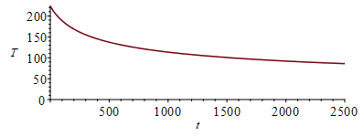
| > | To:=2*Pi*sqrt((R+H)^3/(G*M));To_:=evalf(subs(dat,%));'To_'=subs(SI0,%)*minutes/60;Te_To:=arccos(sqrt((h^2-1)/h))/Pi;Te_:=To_*evalf(subs(eqh_,dat,%));'Te_'=subs(SI0,%)*minutes/60;eqEB:=m*c*dT/dt=Qin-Qout;eqEB:=m*c*dT/dt='Qp'-Qout;eqEB:=m*c*dT/dt='Qp_2'-(epsilon1+epsilon2)*A*sigma*(T^4-Tinf^4);eqEB:=m*c*dT/dt=-(epsilon1+epsilon2)*A*sigma*T^4;eqT:=T(t)=T0/(1+t/tau)^(1/3);eqtau:=tau=m*c/(3*(epsilon1+epsilon2)*A*sigma*T0^3);eqm:=m=rho*A*delta;eqm_:=subs(dat,%);eqtau_:=subs(eqm_,T0=T0_,dat,eqtau);plot(subs(T0=T0_,eqtau_,dat,SI0,rhs(eqT)),t=0..2500,'T'=0..225);T_end:=subs(T0=T0_,eqtau_,dat,SI0,t=2500,rhs(eqT))*K_; |
 |
 |
 |
i.e. the characteristic time is tau=150 s, but we see that the cooling becomes less effective as time passes (at lower temperatures), so that at the end of the eclipse, the plate temperature has only droped from 223 K to 86 K.
| > |