>	restart:#"m13_p21"

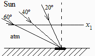
Find the solar constant, E0, based on the following measurements of direct solar irradiation on a horizontal surface at sea level: 940 W/m2 at 20º zenith angle, 860 W/m2 at 40º zenith angle, and 670 W/m2 at 60º zenith angle

Datos:

>	read`../therm_const.m`:read`../therm_proc.m`:read`../therm_eq.m`:with(therm_proc):with(RealDomain):with(plots):with(Statistics):

>	dat:=Const,SI2,SI1:b:=[20,40,60];E:=[940,860,670];

a) Find the solar constant based on sea level irradiance measurements.

August Beer (Germ.) 1852, law of the absorption of light in continuous media is, dI=-C*I*dx, where dx is the optical depth contributed by main gases (N2 and O2), diluted gases (Ar, H2O, CO2, NO2, O3, O), and aerosols (drops of aqueous solutions, and particles).

Integration yields , E(x)=E0exp(x/x0), and near planar atmosphere, x=x1/cos(), where  is the zenith angle of the Sun (=0 if on the vertical direction) and x1 is the atmosphere thickness, the measured irradiation must verify E()=E0exp[x1/(x0cos())], or lnE=lnE0x10/cos(), with x10x1/x0; and we have to fit the data: ln(940)=lnE0x10/cos(20º), ln(860)=lnE0x10/cos(40º), ln(670)=lnE0x10/cos(60º); three equations for two unknowns E0 and x10. The best fitting gives E0=1380 W/m2, not far from the real value E0=1370 W/m2

>	eqBeer:='E(x)=E0*exp(-x/x0)';eqx:=x=x1/cos(beta);eqBeer:='E(beta)=E0*exp(-x1/(x0*cos(beta)))';eqBeer:=lnE=lnE0-x1_0/cos(beta);

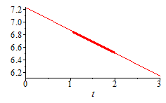
Let us call c_b=1/cos(beta), and make a linear fit.

>

c_b:=evalf([seq(1/cos(beta*Pi/180),beta in b)]);lnE:=[seq(log(E[i]),i=1..3)];pl:=plot([[c_b[1],log(E[1])],[c_b[2],log(E[2])],[c_b[3],log(E[3])]],thickness=3):pol:=LinearFit([1,t],c_b,lnE,t);eqfit1:=lnEfit=op(1,pol)+(op(2,pol)/t)/cos(beta);eqfit2:=Efit=expand(exp(op(1,pol)+(op(2,pol)/t)/cos(beta)));eqfit0:=evalf(subs(beta=0,%));eqfitx:=Efit=expand(exp(op(1,pol)+(op(2,pol)/t)*x));p:=plot(pol,t=0..3):display([p,pl]);

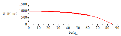
In the original variables:

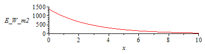
>	pl:=plot([[b[1],E[1]],[b[2],E[2]],[b[3],E[3]]],thickness=3,symbol=BOX):p:=plot(subs(eqfit2,beta=beta_*Pi/180,Efit),beta_=0..90,E_W_m2=0..1500):display([p,pl]);plot(subs(eqfitx,Efit),x=0..10,E_W_m2=0..1500);

Notice the difference between E0=1380 W/m^2, and E1=960 W/m^2 with air-mass AM=1.

>